Differential Gene Expression Tools Research

Abstract

RNA-Seq (named as an abbreviation of "RNA sequencing") is a technology-based sequencing technique which uses next-generation sequencing (NGS) to reveal the presence and quantity of RNA in a biological sample at a given moment, analyzing the continuously changing cellular transcriptome. Differential expression analysis takes the normalised read count data and performs statistical analysis to discover quantitative changes in expression levels between experimental groups. As technology progresses by each year passing, there are now a lot of technological tools available in the Internet that can perform such differential expression analysis. The purpose of our project is to take a closer look at some of these tools, and compare their performances to understand which tools are optimal to utilize. Specifically, the softwares that we are going to focus on are: ABSSeq, voom.limma, PoissonSeq, DESeq2, NOISeq, ttest and edgeR. We are going to compare their performances by looking at parameters such as Area Under the Curve (AOC), False Discovery Rate (FDR), Type I error rate, and Sensitivity.

Background

In genetic research, the understanding of transcriptomes – the set of all RNA transcripts – is crucial for researchers to gain insight into the development of diseases, conditions, or disorders with known genetic etiologies. The goal of the transcriptomic research is to catalogue all species of transcript, including mRNAs, non-coding RNAs & small RNAs and more importantly, to quantify the changing expression levels of each transcript during development and under various environmental and disease conditions. Identifying genes that are differentially expressed is extremely helpful in determining which biological mechanisms could have an effect on a disease or disorder. In the past, researchers primarily used hybridization approaches, such as microarrays, to deduce and quantify these transcriptomes9. Hybridization involves incubating labelled cDNA to microarrays, which while being relatively high throughput and inexpensive, also have limitations such as reliance upon existing knowledge about genome sequence, and limited dynamic range of detection9. Traditionally, researchers used to perform microarrays to analyze genes. However, RNA-Sequencing has recently grown in popularity due to their ability to provide much more precise and accurate measurements, and their potential to cover a wider range of transcripts that haven’t been correlated to an existing genome, while also having extremely low background signal all at a lower cost compared with microarrays.

With the emergence of RNA-sequencing data, countless softwares have been developed to extract information from such data. To process the RNA-sequencing data, a researcher needs to first quality check the reads produced by RNA-seq. For some instances, it is necessary to clean the RNA-seq reads from contamination from adapters during preprocessing. Finally, the researcher analyzes the differentially expressed genes among all the samples. For each step of this process, there are corresponding tools that can be used to help the researchers. In every genetic study using RNA-seq data, researchers must both determine which tools to use and how to precisely use them as there is no single standardized pipeline for differential expression due to the diversity in types of RNA data. Here, we hope to investigate which software is the most efficient and yield the best results by comparing specific tools on both a synthetic dataset and a real life dataset. Because quality control and cleaning of RNA-seq data can only be assessed by computational efficiency and costs, we would want to focus the core of this project on comparing gene differential expression tools. Different tools utilize distinct methods to normalize and calculate the abundance of each gene expressed in each sample, so we would like to test these tools against each other to study which would produce the best results. Overall we include for analysis the following tools: ABSSeq, voom.limma, PoissonSeq, DESeq2, NOISeq, ttest and edgeR, while evaluating their performance on Area Under the Curve (AOC), False Discovery Rate (FDR), Type I error rate, and Sensitivity. The importance of this project is to possibly help future researchers by providing them information about which tools they could utilize for their RNA-seq research for the best results based on the composition of the data and which accuracy metrics need to be controlled.

Dataset

Real life RNA-seq data are hard to interpret and genes determined to be differentially expressed are determined only within a degree of certainty in a normal experiment, we decided to test the tools using a simulated post-alignment dataset, in which we can control variables such as proportion of genes differentially expressed, number of up and down-regulated genes, outliers, and samples per condition. Because it is a synthetic dataset, we can know with full certainty which genes are truly differentially expressed and therefore we can actually calculate accuracy metrics against the truth, which we would not be able to know in a real experiment. We chose to create several datasets with various combinations of number of differentially expressed genes and samples per condition in order to capture the different types of real life genetic data. This will allow us to test, for example, if certain tools work better when there are many differentially expressed genes as opposed to few.

Figure 1. The table above shows the different generated The ‘B’ represents the baseline, ‘P’ represents the Poisson, ‘S’ represents the single outlier, and ‘R’ represents the random outlier. In each simulated study, there are different numbers of differentially expressed genes between the 2 conditions which will be explained more thoroughly below.

In all simulated studies, there are 2, 5 and 10 samples between 2 conditions, denoted by S1 and S2. The simulated studies (left column) have superscripts which represents the number of upregulated DE genes and the subscript represents the number of downregulated DE genes in the second condition (S2). The baseline, single outlier, and random outlier have counts generated from the Negative Binomial distribution whereas Poisson is generated from the Poisson distribution. The ‘single’ outlier fraction is the fraction of genes in a selected single sample where the corresponding count is multiplied with a factor between 5 and 10 — ‘random’ outlier fraction is similar but with a randomly selected sample.

Methods

Creating the Synthetic Data

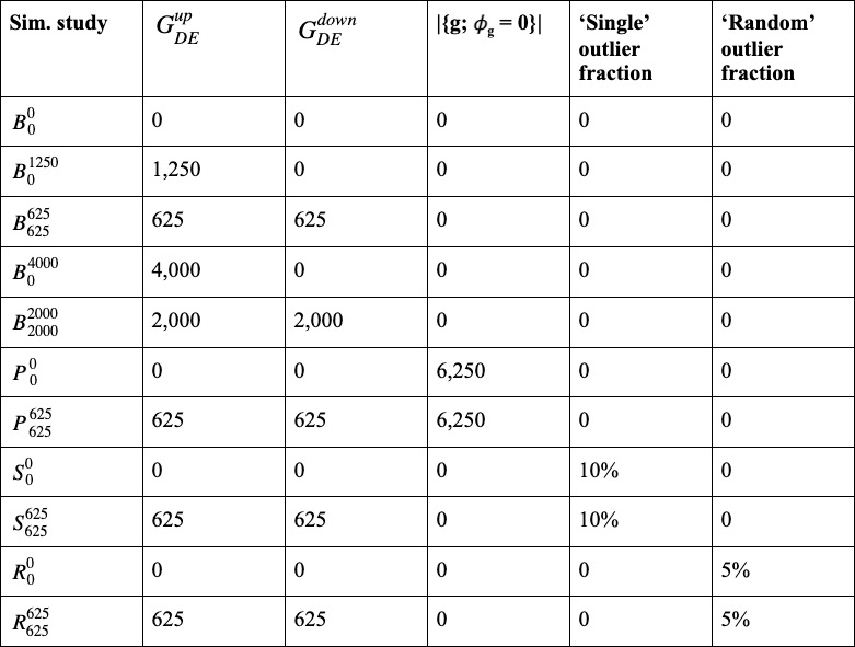
We used compcodeR to investigate the different tools by first creating the synthetic data using the built-in function, generateSyntheticData. For the distinct 11 simulated datasets, we specified the parameters: `n.vars` = 12,500, `samples.per.cond` = 5, `dispersions` = # |{g; 𝜙g = 0}| column in Figure 1. To produce the fraction of differentially expressed genes that is upregulated in S2 compared to S1, `fraction.upregulated` = the ratios shown in Figure 1 (i.e. 0.5 for B625625). For the single outlier fraction datasets, `single.outlier.high.prob` = 0.05 (fraction of single outlier has unusually high counts) and `single.outlier.low.prob` = 0.05 (fraction of single outlier has unusually low counts). As for the random outlier fraction datasets, `random.outlier.high.prob` = 0.025 (fraction of random outliers with unusually high counts) and `random.outlier.low.prob` = 0.025 (fraction of random outliers with unusually low counts).

Performing Differential Expression

For performing tools that were supported by compcodeR, we used the built-in function called `runDiffExp` where we specify the `result.extent` parameter as: DESeq2, edgeR, NOISeq, voom.limma, and ttest. ABSSeq and PoissonSeq, which are not as commonly used, were not supported by compcodeR and needed to be run separately. For both tools, the count matrix was extracted from the compcodeR object for each dataset and labeled to distinguish between conditions based on the number of samples per condition. Both were then run using default parameters and labeled 1 or 0 based on a cutoff value of 0.05 for adjusted p-value.

ABSSeq

This tool performs differential expression analysis of RNAseq data by absolute counts difference between two groups, utilizing Negative binomial distribution and moderating fold-change according to heterogeneity of dispersion across expression level.

voom.limma

This tool performs differential expression analysis of RNAseq data (comparing two conditions) by applying the voom transformation (from the limma package) followed by differential expression analysis with a t-test. Voom precision weights unlock linear model analysis tools for RNA-seq read counts. Then, limma fits a linear model to the expression data for each gene

PoissonSeq

This tool estimates the sequencing depths of experiments using a new method based on Poisson goodness-of-fit statistic, and calculates a core statistic on the basis of a Poisson log-linear model, and then estimates the false discovery date using a modified version of the permutation plug-in method.

DESeq2

This tool performs differential gene expression analysis by estimating the variance-mean dependence in count data using the Negative Binomial Distribution. More specifically, DESeq2 estimates the size factors using the gene counts of the samples, then estimation of dispersion, and lastly performs Negative Binomial Distribution GLM fitting and Wald significance tests. For our purpose, we created a parametric type of fitting of the dispersions to the mean intensity and utilized the Wald test to perform differential gene analysis.

NOISeq

This tool performs differential gene expression analysis of RNA-seq expression data between two conditions without parametric assumptions. NOISeq models the noise distribution of count changes by contrasting fold-change differences and absolute expression differences for all the features in samples within the same condition. NOISeq has 3 main functions: performing quality control of count data, normalization and filter low-counts, and performing differential expression analysis.

ttest

This tool uses the edgeR package to perform differential expression analysis of RNAseq data (comparing two conditions) using a t-test, applied to the normalized counts.

edgeR.exact

This tool performs differential gene expression analysis of RNA-seq expression profiles with biological replication. This R package contains multiple statistical methodology based on the Negative Binomial Distributions, including empirical Bayes estimation, exact tests, generalized linear models, and quasi-likelihood tests. For our investigation, we implemented genewise exact tests for differences in the means between the 2 conditions of negative-binomially distributed counts

Results

For the purpose of a cleaner representation of our research, we chose not to dive too deep in the explanation on this visual represetation. For a more comprehensive analysis of our research, we suggest to take a look at our research report, where we dive in deeper and look at each different dataset. There, we identify the effects from having more or less upregulated and low regulated genes, and how outliers affect the results. We also looked at how a Poisson distributed dataset would perform using the different datasets.
For the purpose of this visual representation, we selected some of the graphs that were outputted from our pipeline that were more representative of our results. Most of researchers are looking for a good Area Under the ROC Curve statistic. We chose to also include Accuracy and FDR, as they also are important in different areas of studies as well.

Area Under the ROC Curve

The ROC curve is a popular graphical tool for comparing the performance of multiple classifiers. The name “ROC” is an acronym for receiver operating characteristics, which comes from communications theory. The overall performance of a classifier is given by the area under the (ROC) curve (AUC). So the larger the AUC the better the classifier.
We can see that generally, with the increasing of samples, the performances of all the tools increase for the AUC metric. This is intuitively predictable, as we get better results if we work with more data. We could observe that DESeq2, edgeR.exact, voom.limma, ttest and PoissonSeq have fairly similar AUC results, having a difference that maxes out at 0.1 depending of the dataset being analyzed.

Accuracy

Accuracy refers to how closely the measured value of a quantity corresponds to its “true” value.
Just like AUC, we can see that across all graphs, it can be observed that as sample size increases, so does the accuracy. We could also again see that except for ABSSeq, all the other tools performed respectively well.

False Discovery Rate

False discovery rate refers to the proportion of significance tests that reject a null hypothesis when it is in fact true
DESeq2, edgeR, voom.limma, and ttest, all rank around 0.5 for false discovery rate with small variance which means that these tools are good at predicting whether a gene is differentially expressed. ABSSeq has a high false discovery rate which means that it doesn’t perform nearly as well as the other tools in terms of predicting whether a gene is truly differentially expressed. Furthermore, almost all tools portray low variances, except for ABSSeq which demonstrates how ABSSeq may not be performing analysis correctly most of the time because of how spread out the data points are from the mean. Similar to ABSSeq, PoissonSeq doesn’t perform as well as the other tools (DESeq2, edgeR, voom.limma, & ttest) as it received False Discovery Rates higher than 0.5, but still performed better than ABSSeq. However, there is a unique trend here where the FDR would decrease as the number of samples increase for PoissonSeq.

Conclusion

As expected, there was no one software that performed better than the others in all of the metrics we measured further proving that researchers need to be particular when choosing what tool to use in a given study. As more general, all-encompassing statistics, the results on AUC and accuracy show that DESeq2 and EdgeR are solid choices for most studies although if runtime is a major factor, as can be the case as RNA extraction becomes cheaper and more available, EdgeR may be the better choice since on average it took many factors less time than DESeq2. Other tools such as voom.limma and ttest performed particularly well on datasets generated with the poisson distribution instead of the negative binomial distribution which is used to simulate variation in the input data. This could indicate that it may be better to use these tools when the data is known to have more of this similar variability. Finally, ABSSeq, which was by far the worst in almost all other circumstances, proved to be the best in terms of False Positive rate in the datasets with zero differentially expressed genes showing that it could be more valuable when the expected number of differentially expressed genes in a study is low since it is more selective when differentiating between genes leading to a lower amount of false positives.

Overall while our research found similar results to previous studies in the past, there is still much more that can be explored in this area especially as this area continues to grow and be improved upon. Furthermore, our findings were mostly observational as it is difficult to quantify and understand why exactly different softwares produce varying results based on the complexity of the statistical methods used across tools. The cleanliness of the synthetic data also needs to be taken into consideration when thinking about the results because real life RNA sequencing data is much messier in practice with many steps being required to even get to differential expression, each with its own variability that can affect results. While we used the random and single outlier functions to attempt to simulate this idea, it may not necessarily translate the same exact way in practice and it would be preferable to test against even more types of diverse real life datasets to validate our results. Finally, there are of course dozens of other softwares that could be tested against but we believe that the tools we chose represented a good mixture of those commonly used in other studies as well as some that take different statistical approaches in order to observe how their use affects the results and help guide decisions in the future on which tools to use.

Again, for a more comprehensive understanding of our findings, we suggest to take a look at our research report, where we have more detailed specifications of our methods and conclusions.

References:

generateSyntheticData